Daily news, dev blogs, and stories from Game Developer straight to your inbox
Sponsored By
Featured Blog | This community-written post highlights the best of what the game industry has to offer. Read more like it on the Game Developer Blogs.
Advanced math in game design: random walks and Markov chains in action
In this article, we’ll analyze two mathematical concepts: Markov chains and random walks.
19 Min Read
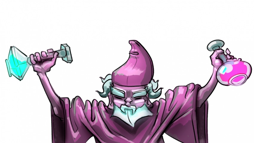
Hello everyone, my name is Lev Kobelev, I am a Game Designer at MY.GAMES. Advanced knowledge of mathematics is rarely considered strictly necessary for game designers — or, if it is required, school level is enough. And that’s true in most cases. But sometimes, knowing certain concepts and methods from advanced mathematics can make life easier and help you look at some problems from a different angle.
In this article, we’ll analyze two mathematical concepts: Markov chains and random walks. I’ll note upfront that this article is more «popular» than «scientific», so, some things about how the formulas are derived will be omitted.
After the theory, we’ll discuss example cases where these tools might come in handy, for example:
The number of chests the player will open if more chests can come out of the chests
The amount of gold to be spent pumping up a sword, if the sword can break
The probability of winning a cash match
Alchemist’s problem
First up, let’s imagine a game where we play as an Alchemist. Our task is collecting ingredients for a new potion:
Ingredient | Location |
Grassweed | Chess Field |
River Meteorites | Space River |
Seirreb | Troll’s Loo |
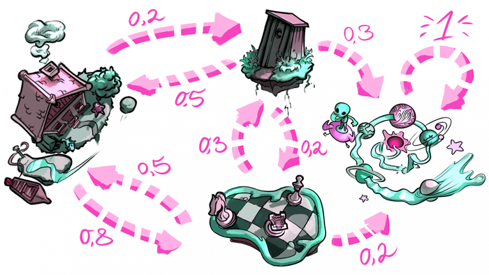
The unique thing about this: roads between our locations can lead us to multiple, randomly selected, destinations.
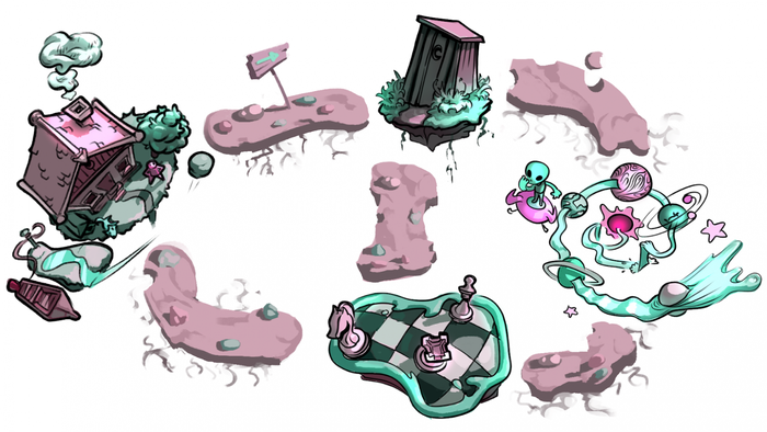
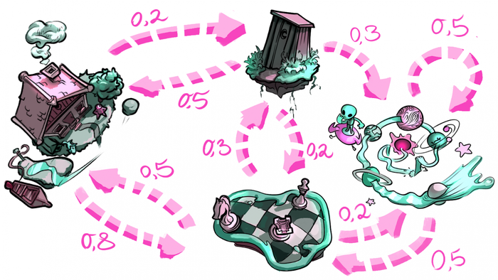
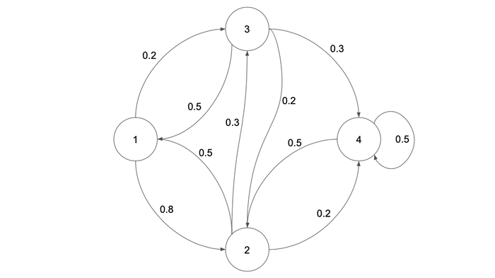
We’ll denote the roads as follows: (location A → location B: the probability of moving from location A to location B):
House → Chess Field: 0.8
House → Troll's Loo: 0.2
Chess field → House: 0.5
Chess Field → Troll's Loo: 0.3
Chess Field → Space River: 0.2
Troll's Loo → House: 0.5
Troll Loo → Chess Field: 0.2
Troll Loo → Space River: 0.3
Space River → Chess Field: 0.5
Space River → Space River: 0.5
Please note: the sum of all destination probabilities from each location equals 1. If the sum is less than 1, then the difference is the probability of transition from A to A. And if it’s more, something definitely went wrong.
The Alchemist goes to get the ingredients. The question: what is the probability that, after two moves, he’ll be at Space River?
There are two possible paths to the river, consisting of two moves:
House → Chess Field → Space River: 0.8 ⋅ 0.2 = 0.16
House → Troll’s Loo → Space River: 0.2 ⋅ 0.3 = 0.06
So, the probability the alchemist will be at the River is 0.22.
Okay, what if we want to know the probability he’ll be at his house after 10 moves? After 100? This takes a lot of calculation, and that’s where Markov chains come to the rescue!
Markov chains
Let’s introduce the following symbols:
S is a finite multitude of states. In our case, this is a multitude of locations: {House, Chess Field, Troll's Loo, Space River}.
Xi is the state after the i-th transition, Xi ∈ S.
Move is a change of state Xi to Xi+1 with a given probability.
Stochastic process is a set of states {X0 , X1 , X2 , ..., Xn−1, Xn}, for example, {House, Chess Field, Space River, ..., House}.
Note: the next state depends only on the current state; it’s as if we don’t know about all the past ones. Such processes are called Markov chains.
If you look closely, you might guess that this is actually a directed graph. Its peaks are locations, that is, elements from the S states’ space. The roads are the edges of the graph, the weights of which are equal to the corresponding probabilities.
Xi / Xi+1 | House | Chess Field | Troll’s Loo | Space River |
House | 0.8 | 0.2 | ||
Chess Field | 0.5 | 0.3 | 0.2 | |
Troll’s Loo | 0.5 | 0.2 | 0.3 | |
Space River | 0.5 | 0.5 |
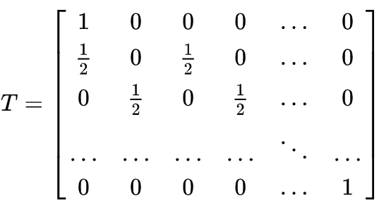
The table shown as a matrix:
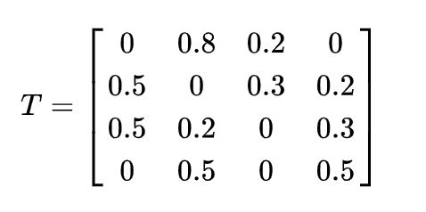
Strictly speaking, we’ve got a matrix of moves, where:
The matrix itself turned out to be square, and, as it reflects all possible moves, the sum of the rows is 1.
Small reminders:
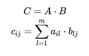
aij is a matrix element, where i is a row number, j is a column number.
You can only sum up matrices one size. In this case, elements with the same index are added.
The product of matrices is defined only if the number of columns of the first matrix is equal to the number of rows of the second. When multiplying the i-th row of the matrix A by the j-th column of B, we get cij, and together they form a new matrix C.
Any random variable (for example, Xi) has a distribution. In our case, we can indicate it as a row vector of N dimension, where N is the cardinality of the S multitude. If the state passes only into itself, it is referred to as absorbing.
Tip:
The calculations for this part of the article can be found on Google Sheets.
The wandering Alchemist
Let’s return to the Alchemist and his adventures. I’ll reiterate: we want to know the probability that he’ll be at his house after a certain number of moves.
In total, we have four locations — therefore, the power S = 4. The Alchemist also starts the journey from home. Here we obtain the distribution of the random variable X0 and denote it as a row vector X0′:
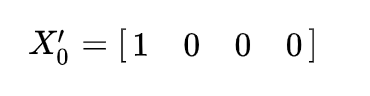
When multiplying X0′ by T, we get X1′ — X1 row vector of distribution :
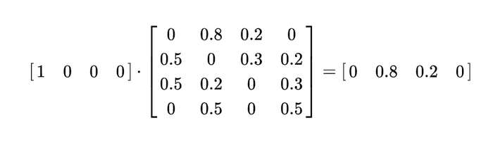
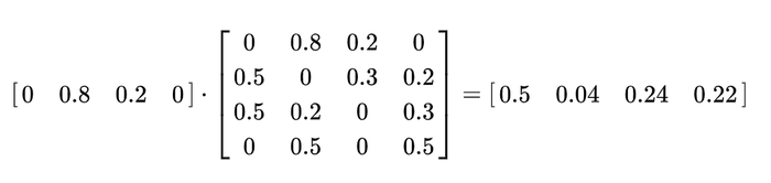
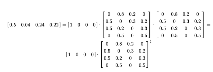
This row vector shows the probability of the Alchemist being in each of the locations after one move. Further, when multiplying X1′ by T, we get X2′, X2 row vector of distribution:
Note that:
Tip:
Matrices can be multiplied in Google Sheets or Excel with the help of = MMULT().
Thus, the distribution per step t is the product of the initial distribution and the transition matrix to the power of t:
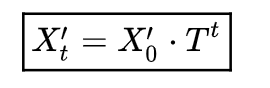
Here, the first element of the resulting row vector is the probability of being home after t moves — problem solved!
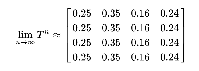
Interesting fact:
The limit Tn at n → ∞ will give the probability of being in state j after an infinite number of steps, where j is the j-th column. This is also called the equilibrium (steady state). The value of the state can also be interpreted as the time that will be spent in it regardless of the initial state. Time in this case is measured as a percentage:
Take me to the river
In practice, we’re more often interested in the probability of an event occurring than in its distribution. And as for the processes, the hitting probability. For example, the probability of hitting subset A of set S.
For convenience, let’s denote the locations through indices:
House
Chess Field
Troll’s Loo
Space River
Suppose that A = {4}, and the initial state i = 1, in this case the hitting probability is the probability he’ll ever get from House to the Space River.
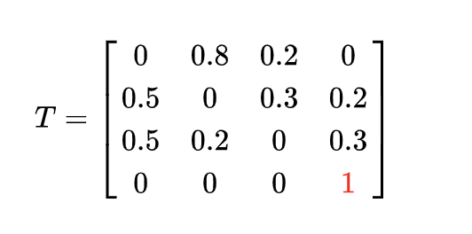
Suppose a weeklong event of raging rivers has started in the game, thus making it impossible for the Alchemist to travel. Now the Space River is an absorbing state, because if the Alchemist goes to it, he will not be able to get out.
The new matrix of moves:
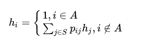
If we suppose that A is an absorbing state, then hi is the absorption probability.
Let's apply the following formula:
Tip on how to work with the formula:
1. Let's go through each state i from the first to the last, denoting them as h with the state index:
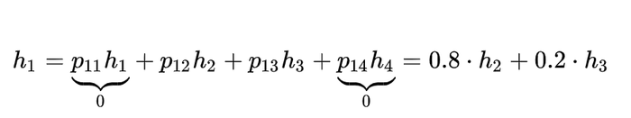
1.1 If i is in set A, hi equals 1. The «inverted letter E» means belonging, and crossed out one means not belonging. For example, i = 1 (that is, a House) is not in A because A = {4}.
1.2 If i is not in set A, we equate i the sum of move probabilities i → j, multiplied by the corresponding hj, which is still unknown to us.
2. We get a set of coupled h, that is, a system of linear equations, where the unknown variables are hi. In a sense, this is a school x.
Let's find each hi using the substitution method, or any other. In tables, this is done using a more complex method. The result should be as small as possible, but at the same time, each value of the system should not be less than 0.
Let's make calculations for h14:
Having done this for each state, we get:
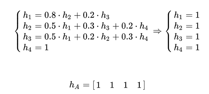
Thus, whatever state the Alchemist starts from, he will definitely end up at the river. Quite expected!
Imminence steps
Additionally, one may often be interested, not so much about the probability of an event, as its expected value. When it comes to random processes, this is the transition time from the initial state to the given one (the expected hitting time). Time is an abstraction that can be a step, an action, whatever we want. The hitting time is also often referred to as the reach time. If A is an absorbing state, the time is also called the absorbing time.
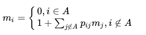
Let’s use the following formula:
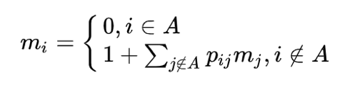
And again, the result should be as small as possible, but at the same time, each value of the system should not be less than 0.
Question: after how many moves will the Alchemist get stuck in the river?
Let's write a calculation for m1:
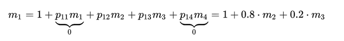
Having done so for each state, we get:
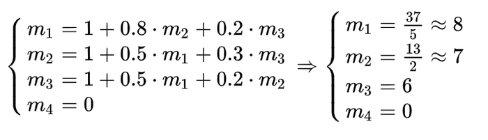
So, it turns out that after about 8 moves the Alchemist will get stuck in the river — 37/5 is closer to 7, but let's be optimistic (and, as practice shows, it is better to round up numbers).
What we’ve hidden behind the scenes:
I did not show the deriving of all the formulas. Nevertheless, in the following sections, arguments will be given on the derivation of similar formulas — they can help in independent reasoning.
Randoms walks
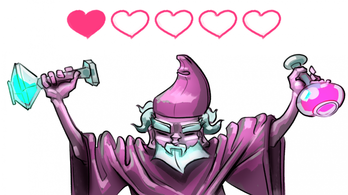
Imagine the Alchemist is now making magical potions, and consider the following:
The Alchemist has an initial health of 1 and maximum health of 5
He can produce a regeneration potion that restores +1 health
Sometimes he makes a bad potion; it reduces health -1
The probabilities of making a good and bad potion are equal
At a health equal to 0, the Alchemist dies, and at 5, the round ends
Question: how soon will the game end? That is, will the Alchemist perish or be able to fully restore his health?
Here, random walks come to our aid, (these can often be considered as a special case of Markov chains). Sure, not every Markov chain is a random walk or vice versa, because, to illustrate the point, random walks can have an infinite number of states.
In simple terms, a random walk is a mathematical object that describes a path consisting of a set of random steps. It’s important to understand that the path is some kind of abstract entity that may not actually have anything to do with the real path.
Here, speaking in mathematical terms, a simple limited symmetrical random walk is described, because you can only move to neighboring values – for example, you cannot reduce health immediately from 2 to 0. At the same time, it is limited both from below and from above, and the probabilities of reducing and increasing are equal.
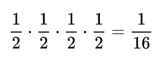
Let’s consider the case of full health recovery. In order to try and find a pattern, let's start with the simple scenarios. In the most basic one, he drinks 4 correctly made potions in a row. Here, we get the probability:
And if one potion takes 1 health point? For convenience, let’s assume all the green colors in formulas, graphs, and figures are bad potions, like some toxic colors, and red ones are good, like a bright heart.
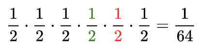
A bad potion must be offset by a good one to restore health to the max. There are only 3 such scenarios, depending on when we drink the bad potion:
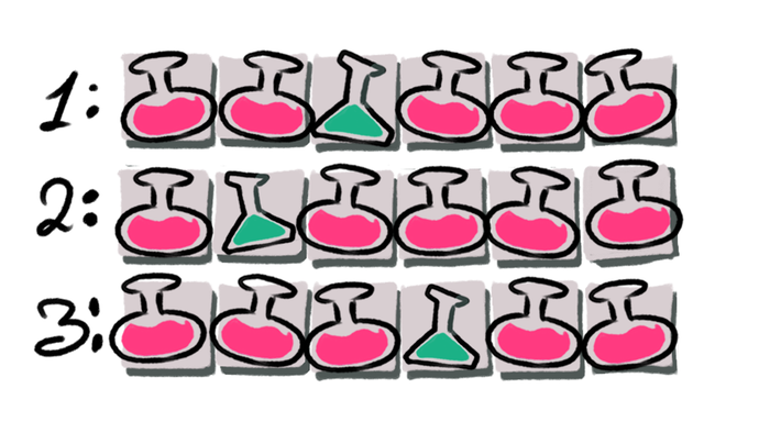
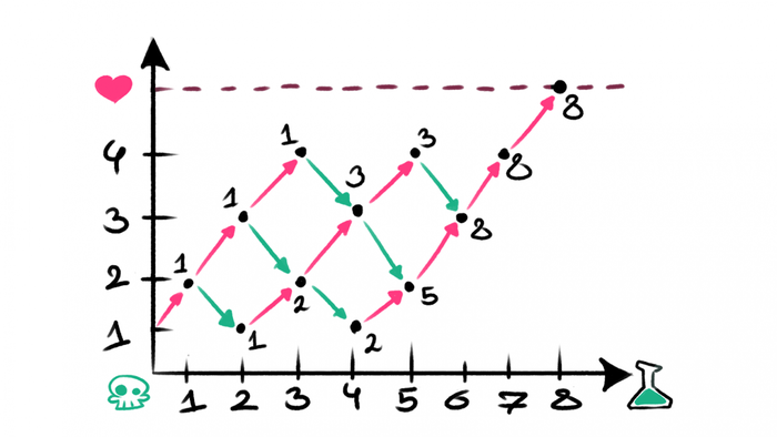
As the number of bad potions grows, so does the number of possible options. One option for counting them is to represent everything in the form of a graph.
For 8 potions (2 of which are bad), we get 8 possible paths:
There are two questions:
How many potions can we take? 5? 12?
Is it possible to calculate this analytically, without using a graph?
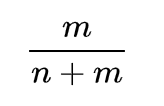
We understand we need to restore 4 health points (if we start from 1 and the maximum is 5) by drinking n number of potions. In this case, we get:
m = 4, as health that needs to be restored
p, the number of good potions;
(n - p), the number of bad potions.

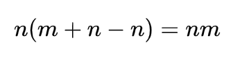
Thus, if p is odd, he won’t be able to fully restore his health with this number of potions. Knowing the number of good potions, we can easily find bad ones. For example, for a total number of 8 we get:
Any attempt to restore health is a set of potions, such as {good, bad, good, ..., bad}. In our case, such a set consists of 8 potions, 2 of which are bad. So, to get our answer, it’s sufficient to calculate the number of combinations without repetitions.
Let me remind you the formula:
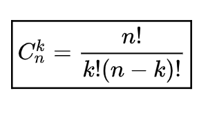
We will get:
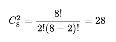
But 28 is much bigger than 8! Have we missed something on the graph?
No, on the contrary: when we counted through combinations, we took into account too much, namely, the early cases of death and restoring life.
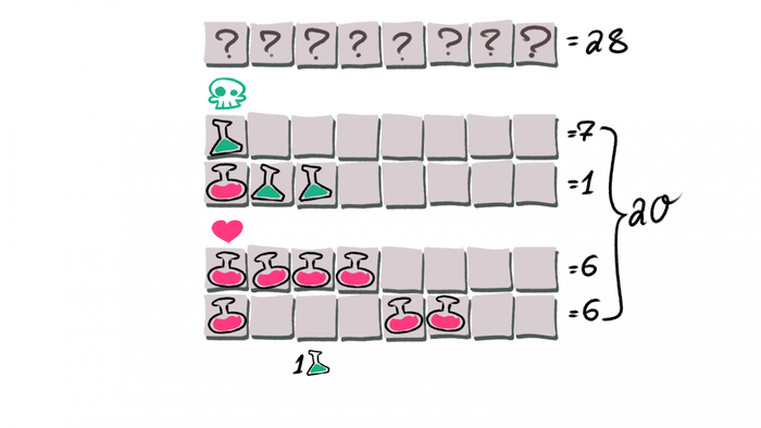
Early deaths:
The player initially drinks a bad potion.
The player drinks a good potion followed by two bad potions.
Early recovery:
The player drinks 4 good potions in a row.
The player drinks a good one, then a bad one, then 4 good ones.
If we count all such combinations, we get exactly 20 extra cases. And as a result, 8 possible.
No one can guarantee that such a chain will be finite, because a bad potion can alternate with a good one for an infinitely long time. From here we get the following amount, which describes the probability of restoring health:
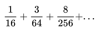
It’s easy to see that this is almost an ordinary infinitely decreasing progression, the sum of which we can find:
Let's take it on faith that we cannot get lost somewhere in space and constantly alternate drinking good and bad potions, and if that’s taken to be true, it means the probability of losing the Alchemist is as follows:
What was left out behind the scenes:
1. The denominators of the fractions are the probability of (1/2)n, where n is the number of potions in total.
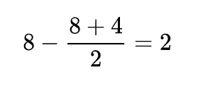
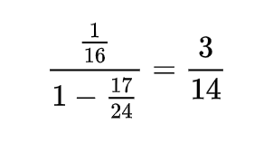
2. The application of the BGP formula to almost BGP is not entirely correct, because the ratio of two adjacent fractions is different, which contradicts the essence of BGP. However, we can calculate the average and get the result of 17/24.
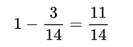
3. To find the probability of the Alchemist’s death, we can do exactly the same as for the probability of a complete recovery, which will give us 11/14.
General case
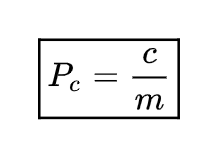
Let the initial health of our Alchemist be current (c) and the maximum health be max (m). In this case, if c is zero, then the probability of restoring health is 0, and if m, it’s 1. If c lies somewhere in between, then the probability will be the sum on the left or right:
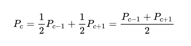
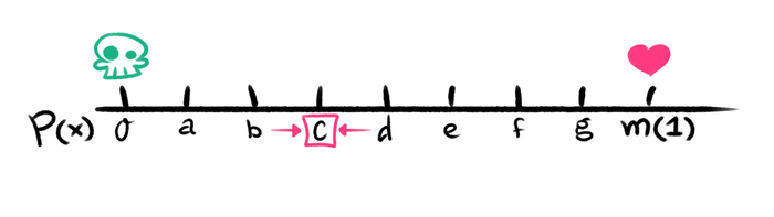
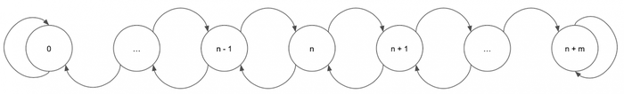
From here we can get a system of linear equations, where the unknowns are the probability of restoring his health if you start from a certain position. For convenience, let's put denominations on the numerical axis and note the probabilities (ends) known to us. We get:
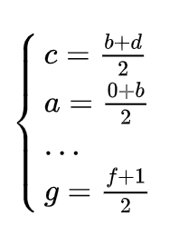
Having solved this system of equations, we will get:
If we return to our case, where c = 1 and m = 5, we get 1/5, which is almost the same as 3/14 (the absolute difference is 0.014).
Having done the same operation, but changing the edges, we get a probability of ⅘, which means that the Alchemist has no chance of being in a superposition between death and life.
Moreover, if we consider that after reaching some maximum, health continues to recover instead of the round ending, we get:
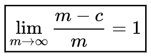
Thus, no matter how many potions the Alchemist drinks, he will die sooner or later.
How many potions will he have to drink?
As mentioned earlier, in random processes, we are often interested in the transition time from one state to another. Obviously, in our case, time is the number of potions consumed. So how many potions do you need to drink to fully restore your health?
It’s logical that the extreme values are zero, and the n-th value is the sum of neighboring ones and one more potion, due to the linearity of the value:
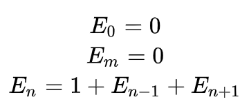
We’ll omit the solution of this math expression, since it will not be possible to solve it through the system. We’ll have to turn to methods for solving recursive equations, and this is not our topic. We get:
Curious facts:
1. The probabilities to recover completely, initially with n, form an arithmetic progression.
2. The set of transition time is a string from Pascal's triangle with number m, but with zeros on the edges.
If we return to the fact that overhealing is possible, we get:
A hint where this infinity comes from:
Let’s leave out the strict definition of the limit. Let m be infinity. Infinity is something huge: we can subtract, add, multiply using it — and still get infinity. (Although sometimes there are exceptions!)
You can drink an infinite number of potions, but die anyway.
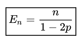
However, it’s quite possible that the probability of a bad potion is higher than a good one (p), which is quite logical for Alchemists. In this case, we get:
What we left behind the scenes:
Solving recursive expressions.
Derivation of the formula for asymmetric walks.
Real cases
It's time to get down to a little practice. When does all this come in handy?
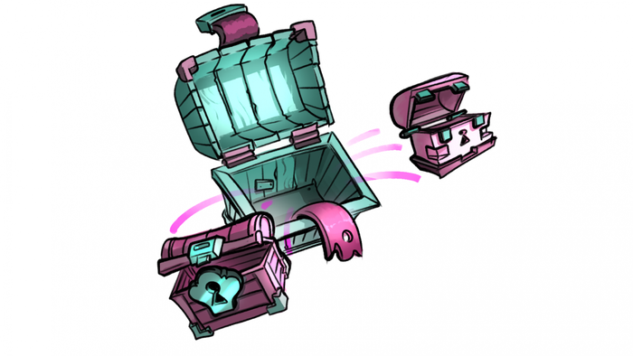
Chests from a chest from a chest...
Suppose the game has the following chest mechanics:
The player initially has 1 chest.
With a probability of 0.4, 2 of the same will come out of it.
There’s a probability of 0.6 that nothing will come out of a chest.
Question: How many chests will one player open on average?
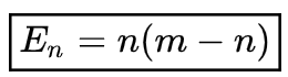
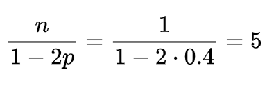
We can assume that n is the current number of chests, which is initially equal to 1, and each action either increases n by 1 or decreases it by 1. The increase by 1 is due to the fact that the player seems to have lost 1 chest, but received 2 new ones. The conditions fit very well with the concept of wandering. Therefore, we simply apply the formula:
Sword sharpening
Suppose the game has the following sword upgrade mechanic:
The player initially has a level 1 sword, currentLevel = 1.
Maximum level = 4.
The player can try to level up the sword. However, in the process, the sword may break and lower its level:
Question: how many coins will a player spend on average to upgrade a sword to the maximum level?
Let's imagine the mechanics as a graph, the vertices of which are the levels, and the edges are the probability of improvement:
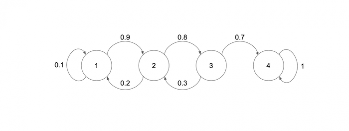
This is a regular Markov chain, and you just need to find m1 with A = {4}, that is, the average number of steps from level 1 to level 4. Let's use the formula:
We get: m1 ≈ 4.72, average cost of improvement = 20, and we just need to multiply them. Thus, on average, a player will spend about 94 coins to upgrade a sword from level 1 to level 4.
A quick question: is it fair to simply take the average price of an improvement like this?
Gambler’s ruin
Let the game have the following match mechanics:
There are two players who have n and m coins.
Players toss a coin one by one:
Players can play as long as both strictly have more than 0 coins.
Question: What is the probability that the first player will lose?
Interestingly, these conditions fit both the Markov chain and random walks. Let’s consider the random walks of the first player:
Moves have a probability of 0.5, because we just flip a coin, except for the extreme ones, they have 1.
The walk graph can be easily transferred to a transition matrix:
So, we can operate both with formulas for Markov chains and for random walks.
Here we get the probability of the second player’s win:
This is also the probability of the first player’s loss.
Additionally, we can calculate the number of flips:
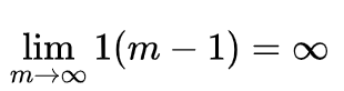
If we assume that the second player is a casino with an infinite supply of money, then the first one will lose sooner or later, although before that, he will make an infinite number of throws.
Conclusion
Much has been left out of the whole picture, but it seems that we managed to cover the primary topics here. Thanks for reading, I hope this can show designers some new tools for solving certain problems, and perhaps this post positively strained and trained some brains for a few readers.
Oh, yes, all this could be calculated using the Monte Carlo method — but first of all, that’d be boring, and second, it’s useful to know what is behind the results, and not take them for granted. Moreover, one needs to be able to write simple scripts!
Do not be afraid of mathematics, evolve, and make good games!
Bibliography
Ian Schreiber, Brenda Romero. Game Balance. 2022.
Images by shabbyrtist
Read more about:
Featured BlogsAbout the Author(s)
You May Also Like